Bollinger Bands using R

Bollinger Plots are a very good way of providing technical information on plausible Buy or Sell on a particular security. They are based on moving averages and thus are simple to create

However, there are 2 parameters that are inputs to the Bollinger Band
1) The period of days considered for calculating the moving average
Most of the analysts use a 20 day plot, but you can use any period based on the security. e.g. A highly liquid security with high volatility should have a lower period.

The R script can be downloaded here

# Bollinger Bands

Ticker = 'AAPL'

URL = paste(c('http://real-chart.finance.yahoo.com/table.csv?s=',Ticker,'&a=01&b=01&c=2015&d=04&e=10&f=2015&g=d&ignore=.csv'),collapse="")

Prices = read.csv(URL)

Prices = Prices[,c(1,5)]

# Simple moving average of a vector of price and the number of days

getMovingAverage = function(dataVector,periodDays,method){

  dataVectorOutput = dataVector

  lengthofVector = length(dataVector)

  for(start in 1:lengthofVector)

  {

    if(start < periodDays)

    {

      dataVectorOutput[start] = NA

    }

    else

    {

      if(method=="mean")  dataVectorOutput[start] = mean(dataVector[start-periodDays:start])

      else if(method=="sd") dataVectorOutput[start] = sd(dataVector[start-periodDays:start])

    }   

  }

  return(dataVectorOutput)

}



dataVectorOutputMean = getMovingAverage(Prices$Close,20,"mean")

dataVectorOutputSD = getMovingAverage(Prices$Close,20,"sd")

Prices$Middle = dataVectorOutputMean

Prices$Upper = dataVectorOutputMean + dataVectorOutputSD * 2

Prices$Lower = dataVectorOutputMean - dataVectorOutputSD * 2



#Remove all the NULLS

Prices = Prices[!is.na(Prices$Middle),]



# Change the date to something that ggplot will understand

Prices$Date = as.POSIXct(as.character(Prices$Date),"%Y-%m-%d")



# Plot the Bollinger

library(ggplot2)

g = ggplot(Prices,aes(Date,Close,group=1)) + geom_line()

g = g + geom_line(data=Prices,aes(Date,Upper,group="Upper Bollinger",color="Upper Bollinger"),size=1)

g = g + geom_line(data=Prices,aes(Date,Middle,group="Middle Bollinger",color="Middle Bollinger"),size=1)

g = g + geom_line(data=Prices,aes(Date,Lower,group="Lower Bollinger",color="Lower Bollinger"),size=1)

g = g + xlab("Date") + ylab("Prices")

g

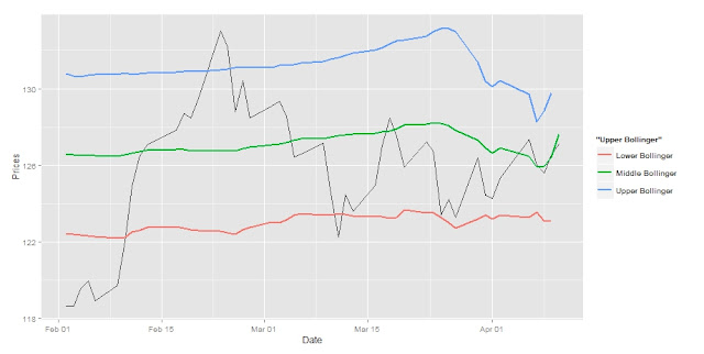
A Sample plot for the AAPL Stock was created using the above script